Feature Engineering

 Feature Engineering is the way of extracting features from data and transforming them into formats that are suitable for Machine Learning algorithms.

It is divided into 3broad categories:-

Feature Selection: All features aren't equal. It is all about selecting a small subset of features from a large pool of features. We select those attributes which best explain the relationship of an independent variable with the target variable. There are certain features which are more important than other features to the accuracy of the model. It is different from dimensionality reduction because the dimensionality reduction method does so by combining existing attributes, whereas the feature selection method includes or excludes those features.
The methods of Feature Selection are Chi-squared test, correlation coefficient scores, LASSO, Ridge regression etc.

Feature Transformation: It means transforming our original feature to the functions of original features. Scaling, discretization, binning and filling missing data values are the most common forms of data transformation. To reduce right skewness of the data, we use log.

Feature Extraction: When the data to be processed through an algorithm is too large, it’s generally considered redundant. Analysis with a large number of variables uses a lot of computation power and memory, therefore we should reduce the dimensionality of these types of variables. It is a term for constructing combinations of the variables. For tabular data, we use PCA to reduce features. For image, we can use line or edge detection.

We start with this data-set from MachineHack.
We will first import all the packages necessary for Feature Engineering.

import pandas as pd
import numpy as np
import matplotlib.pyplot as plt
import datetime

We will load the data using pandas and also set the display to the maximum so that all columns with details are shown:

pd.set_option('display.max_columns', None)data_train = pd.read_excel('Data_Train.xlsx')data_test = pd.read_excel('Data_Test.xlsx')

Before we start pre-processing the data, we would like to store the target variable or label separately. We will combine our training and testing data-sets, after removing the label from the training dataset. The reason why we are combining train and test data-sets is that Machine Learning models aren’t great at extrapolation, ie, ML models aren’t good at inferring something that has not been explicitly stated from existing information. So, if the data in the test set hasn’t been well represented, like in training set, the predictions won’t be reliable.

price_train = data_train.Price  # Concatenate training and test sets data = pd.concat([data_train.drop(['Price'], axis=1), data_test])

This is the output we get after data.columns

Index(['Airline', 'Date_of_Journey', 'Source', 'Destination', 'Route','Dep_Time', 'Arrival_Time', 'Duration', 'Total_Stops',
'Additional_Info', 'Price'], dtype='object')

To check the first five rows of the data, type data.head() .

To see the broader picture we use data.info() method.

<class 'pandas.core.frame.DataFrame'>
Int64Index: 13354 entries, 0 to 2670
Data columns (total 10 columns):
Airline            13354 non-null object
Date_of_Journey    13354 non-null object
Source             13354 non-null object
Destination        13354 non-null object
Route              13353 non-null object
Dep_Time           13354 non-null object
Arrival_Time       13354 non-null object
Duration           13354 non-null object
Total_Stops        13353 non-null object
Additional_Info    13354 non-null object
dtypes: int64(1), object(10)
memory usage: 918.1+ KB

To understand the distribution of our data, use data.describe(include=all)

We would like to analyse the data and remove all the duplicate values.

data = data.drop_duplicates()

We’d want to check for any null values in our data, therefore, data.isnull.sum() .

Airline            0
Date_of_Journey    0
Source             0
Destination        0
Route              1
Dep_Time           0
Arrival_Time       0
Duration           0
Total_Stops        1
Additional_Info    0
Price              0
dtype: int64

Therefore, we use the following code to remove the null value.

data = data.drop(data.loc[data['Route'].isnull()].index)

Airlines

Let’s check the Airline column. We notice that it contains categorical values. After using data['Airline'].unique() , we notice that the values of the airline are repeated in a way.

We first want to visualize the column:

sns.countplot(x='Airline', data=data)plt.xticks(rotation=90)

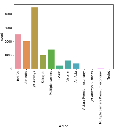
This visualization helps us understand that there are certain airlines which have been divided into two parts. For example, Jet Airways had another part called Jet Airways Business. We would like to combine these two categories.

data['Airline'] = np.where(data['Airline']=='Vistara Premium economy', 'Vistara', data['Airline'])data['Airline'] = np.where(data['Airline']=='Jet Airways Business', 'Jet Airways', data['Airline'])data['Airline'] = np.where(data['Airline']=='Multiple carriers Premium economy', 'Multiple carriers', data['Airline'])

This is how our values in the column will look now.

Flight’s Destination

The same goes with Destination. We find that Delhi and New Delhi have been made two different categories. Therefore, we’ll combine them into one.

data['Destination'].unique()data['Destination'] = np.where(data['Destination']=='Delhi','New Delhi', data['Destination'])

Date of Journey

We check this column, data['Date_of_Journey'] and find that the column is in this format:-

24/03/2019
1/05/2019

This is just raw data. Our model cannot understand it, as it fails to give numerical value. To extract useful features from this column, we would like to convert it into weekdays and months.

data['Date_of_Journey'] = pd.to_datetime(data['Date_of_Journey'])OUTPUT
2019-03-24
2019-01-05

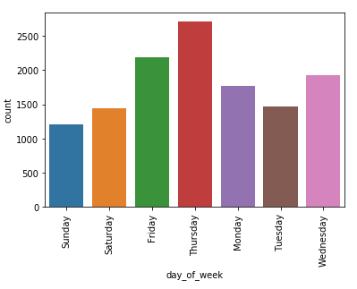
And then to get weekdays from it

data['day_of_week'] = data['Date_of_Journey'].dt.day_name()OUTPUT
Sunday
Saturday

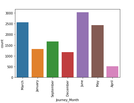
And from Date_of_Journey, we will also get the month.

data['Journey_Month'] = pd.to_datetime(data.Date_of_Journey, format='%d/%m/%Y').dt.month_name()OUTPUT
March
January

Departure Time of Airlines

The time of departure is in 24 hours format(22:20), we would like to bin it to get insights.

We will create fixed-width bins, each bin contains a specific numeric range. Generally, these ranges are manually set, with a fixed size. Here, I have decided to group hours into 4 bins. [0–5], [6–11], [12–17] and [18–23] are the 4 bins. We cannot have large gaps in the counts because it may create empty bins with no data. This problem is solved by positioning the bins based on the distribution of the data.

data['Departure_t'] = pd.to_datetime(data.Dep_Time, format='%H:%M')a = data.assign(dept_session=pd.cut(data.Departure_t.dt.hour,[0,6,12,18,24],labels=['Night','Morning','Afternoon','Evening']))data['Departure_S'] = a['dept_session']

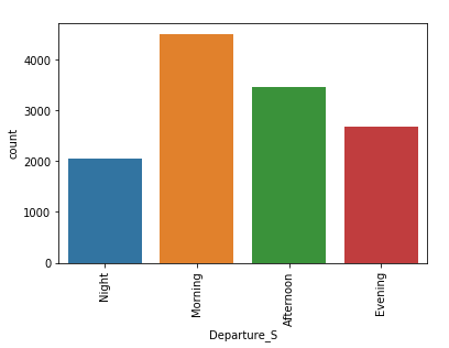
We fill the null values with “night” in the ‘Departure_S’ column.

data['Departure_S'].fillna("Night", inplace = True)

Duration

Our duration column had time written in this format 2h 50m . To help machine learning algorithm derive useful insights, we will convert this text into numeric.

duration = list(data['Duration'])for i in range(len(duration)) :
    if len(duration[i].split()) != 2:
        if 'h' in duration[i] :
            duration[i] = duration[i].strip() + ' 0m'
        elif 'm' in duration[i] :
            duration[i] = '0h {}'.format(duration[i].strip())dur_hours = []
dur_minutes = []  
 
for i in range(len(duration)) :
    dur_hours.append(int(duration[i].split()[0][:-1]))
    dur_minutes.append(int(duration[i].split()[1][:-1]))
     
 
data['Duration_hours'] = dur_hours
data['Duration_minutes'] =dur_minutesdata.loc[:,'Duration_hours'] *= 60data['Duration_Total_mins']= data['Duration_hours']+data['Duration_minutes']

The result we will now get is continuous in nature.

After visualizing data, it makes sense to delete rows which duration less than 60 mins.

# Get names of indexes for which column Age has value 30indexNames = data[data.Duration_Total_mins < 60].index# Delete these row indexes from dataFramedata.drop(indexNames , inplace=True)

We will drop the columns which had noise or had texts, which would not help our model. We have transformed these into newer columns to get better insights.

data.drop(labels = ['Arrival_Time','Dep_Time','Date_of_Journey','Duration','Departure_t','Duration_hours','Duration_minutes'], axis=1, inplace = True)

Dummy Variables

We have engineered almost all the features. We have dealt with missing values, binned numerical data, and now it’s time to transform all variables into numeric ones. We will use, get_dummies() to the transformation.

cat_vars = ['Airline', 'Source', 'Destination', 'Route', 'Total_Stops',
       'Additional_Info', 'day_of_week', 'Journey_Month', 'Departure_S' ]
for var in cat_vars:
    catList = 'var'+'_'+var
    catList = pd.get_dummies(data[var], prefix=var)
    data1 = data.join(catList)
    data = data1
    
data_vars = data.columns.values.tolist()
to_keep = [i for i in data_vars if i not in cat_vars]data_final=data[to_keep]