Skewness
It is the degree of distortion from the symmetrical bell curve or the normal distribution. It measures the lack of symmetry in data distribution.
It differentiates extreme values in one versus the other tail. A symmetrical distribution will have a skewness of 0.
There are two types of Skewness: Positive and Negative

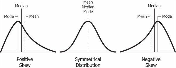
Positive Skewness means when the tail on the right side of the distribution is longer or fatter. The mean and median will be greater than the mode.
Negative Skewness is when the tail of the left side of the distribution is longer or fatter than the tail on the right side. The mean and median will be less than the mode.
So, when is the skewness too much?
The rule of thumb seems to be:
- If the skewness is between -0.5 and 0.5, the data are fairly symmetrical.
- If the skewness is between -1 and -0.5(negatively skewed) or between 0.5 and 1(positively skewed), the data are moderately skewed.
- If the skewness is less than -1(negatively skewed) or greater than 1(positively skewed), the data are highly skewed.
Example
Let us take a very common example of house prices. Suppose we have house values ranging from $100k to $1,000,000 with the average being $500,000.
If the peak of the distribution was left of the average value, portraying a positive skewness in the distribution. It would mean that many houses were being sold for less than the average value, i.e. $500k. This could be for many reasons, but we are not going to interpret those reasons here.
If the peak of the distributed data was right of the average value, that would mean a negative skew. This would mean that the houses were being sold for more than the average value.
Kurtosis
Kurtosis is all about the tails of the distribution — not the peakedness or flatness. It is used to describe the extreme values in one versus the other tail. It is actually the measure of outliers present in the distribution.
High kurtosis in a data set is an indicator that data has heavy tails or outliers. If there is a high kurtosis, then, we need to investigate why do we have so many outliers. It indicates a lot of things, maybe wrong data entry or other things. Investigate!
Low kurtosis in a data set is an indicator that data has light tails or lack of outliers. If we get low kurtosis(too good to be true), then also we need to investigate and trim the dataset of unwanted results.

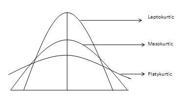
Mesokurtic: This distribution has kurtosis statistic similar to that of the normal distribution. It means that the extreme values of the distribution are similar to that of a normal distribution characteristic. This definition is used so that the standard normal distribution has a kurtosis of three.
Leptokurtic (Kurtosis > 3): Distribution is longer, tails are fatter. Peak is higher and sharper than Mesokurtic, which means that data are heavy-tailed or profusion of outliers.
Outliers stretch the horizontal axis of the histogram graph, which makes the bulk of the data appear in a narrow (“skinny”) vertical range, thereby giving the “skinniness” of a leptokurtic distribution.
Platykurtic: (Kurtosis < 3): Distribution is shorter, tails are thinner than the normal distribution. The peak is lower and broader than Mesokurtic, which means that data are light-tailed or lack of outliers.
The reason for this is because the extreme values are less than that of the normal distribution.


Comments
Post a Comment